Metamodel

This page describes the metamodel EOS parametrization and its implementation in jester.

General background

The metamodel, or a ‘model-of-a-model’, is a model for the homogeneous nucleonic EOS, introduced and described in Refs. [1] and [2]. It describes nuclear matter with different isoscalar (is) density

(1)\[n_0 = n_n + n_p\]

(which we will also denote simply by \(n\) below) and isovector (iv) density

(2)\[n_1 = n_n - n_p\]

where \(n_n\) and \(n_p\) are the neutron and proton number densities, respectively. We also define the asymmetry parameter

(3)\[\delta = n_1/n_0\]

which quantifies the isospin asymmetry of nuclear matter. The two possible extreme values of \(\delta\) describe particular types of nuclear matter:

• Symmetric nuclear matter (SNM) with \(\delta = 0\) (i.e., \(n_n = n_p\)) and

• Pure neutron matter (PNM) with \(\delta = 1\) (i.e., \(n_p = 0\)).

The energy density is the sum of a kinetic and a potential term

(4)\[e_{\rm{MM}}(n, \delta) = t^*(n, \delta) + e^{\rm{pot}}(n, \delta)\]

In the metamodel, the potential energy of this matter can be expanded as follows:

(5)\[e^{\rm{pot}}(n, \delta) = e_{\rm{is}}(n) + \delta^2 e_{\rm{iv}}(n) + \mathcal{O}(\delta^4)\]

where \(e_{\rm{is}}(n)\) and \(e_{\rm{iv}}(n)\) are the isoscalar and isovector contributions to the energy per nucleon, respectively. Note that \(n_1\) enters implicitly in the asymmetry parameter \(\delta\). Often, the isovector energy is also called the symmetry energy. We define the saturation density \(n_\mathrm{sat}\) of symmetric nuclear matter as the density at which the symmetric matter pressure reaches zero.

The potential energy, in the metamodel, is modeled as a Taylor expansion around saturation density, and the expansion is truncated at some order. In practice, the expansion parameter is \(x\), defined as:

(6)\[x = \frac{n - n_\mathrm{sat}}{3 n_\mathrm{sat}}\]

This Taylor expansion introduces the nuclear empirical parameters (NEPs) as the coefficients of the expansion, which are related to physical properties of nuclear matter at saturation density. Using these definitions, most equations and metamodel source code is written as function of \(x\) and \(\delta\) instead of \(n_0\) and \(n_1\), as this makes the equations more compact and easier to read. Note that this implies that

(7)\[\frac{n}{n_{\rm{sat}}} = 1 + 3x\]

Which is a useful relation to have when deriving the equations below. Moreover, we can also easily see that

(8)\[\delta = 1 - 2 Y_p\]

where \(Y_p\) is the proton fraction, defined as \(Y_p = n_p/n\).

The Taylor expansions in the original metamodel paper are given by:

(9)\[\begin{split}e_{\rm{is}} &= E_\mathrm{sat} + \tfrac{1}{2} K_\mathrm{sat} x^2 + \tfrac{1}{3!} Q_\mathrm{sat} x^3 + \tfrac{1}{4!} Z_\mathrm{sat} x^4 + \ldots \\ e_{\rm{iv}} &= E_\mathrm{sym} + L_\mathrm{sym} x + \tfrac{1}{2} K_\mathrm{sym} x^2 + \tfrac{1}{3!} Q_\mathrm{sym} x^3 + \tfrac{1}{4!} Z_\mathrm{sym} x^4 + \ldots\end{split}\]

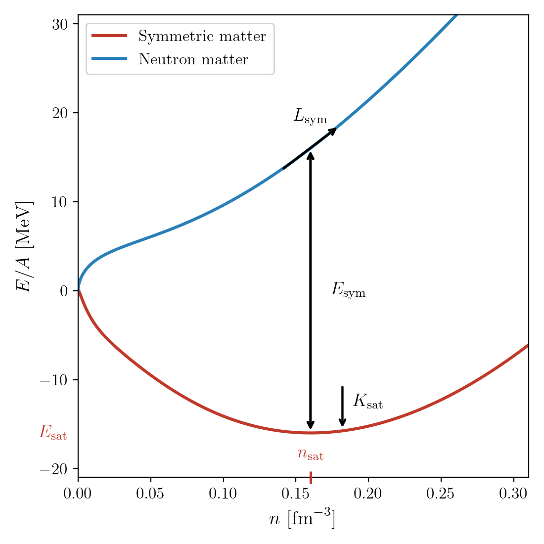
The figure below shows an example of the energy per nucleon \(E/A\) for symmetric nuclear matter and pure neutron matter computed from the metamodel with fiducial NEP values.

(Source code, png, hires.png, pdf)

Energy per nucleon \(E/A\) for symmetric nuclear matter (\(\delta = 0\), red) and pure neutron matter (\(\delta = 1\), blue) computed from the meta-model with fiducial NEP values (\(E_\mathrm{sat} = -16\,\mathrm{MeV}\), \(K_\mathrm{sat} = 230\,\mathrm{MeV}\), \(E_\mathrm{sym} = 32\,\mathrm{MeV}\), \(L_\mathrm{sym} = 60\,\mathrm{MeV}\)).

Below, we explain how both the kinetic and potential energy terms are modeled in jester in more detail.

Kinetic energy

In the metamodel approach, the kinetic energy is modeled using a nonrelativistic free Fermi gas (FG) and by taking into account the effective mass due to the momentum-dependent nuclear interaction (see Section IIIA in Ref. [1] for details). The kinetic energy per nucleon is then given by:

(10)\[\begin{split}t_0(x, \delta) = \frac{t_{\rm{sat}}}{2} (1+3x)^{2/3} \big[ f^{\rm{FG}}(\delta) &+ (1+3x) f^*(\delta) \\ &+ (1+3x)^2 f^{**}(\delta) + (1+3x)^3 f^{***}(\delta) \big]\end{split}\]

where the constant \(t_{\rm{sat}}\) is defined as

(11)\[t_{\rm{sat}} = \frac{3 \hbar^2}{10m} \left( \tfrac{3}{2} \pi^2 n_{\rm{sat}} \right)^{2/3}\]

\(m\) is the nucleonic mass, and the auxiliary functions \(f^{\rm{FG}}\), \(f^*\), \(f^{**}\), and \(f^{***}\) are defined as

(12)\[\begin{split}f^{\rm{FG}}(\delta) &= (1 + \delta)^{5/3} + (1 - \delta)^{5/3} \\ f^*(\delta) &= (\kappa_{{\rm sat}} + \kappa_{{\rm sym}}\delta)(1 + \delta)^{5/3} + (\kappa_{{\rm sat}} - \kappa_{{\rm sym}}\delta)(1 - \delta)^{5/3} \\ f^{**}(\delta) &= (\kappa_{{\rm sat},2} + \kappa_{{\rm sym},2}\delta)(1 + \delta)^{5/3} + (\kappa_{{\rm sat},2} - \kappa_{{\rm sym},2}\delta)(1 - \delta)^{5/3} \\ f^{***}(\delta) &= (\kappa_{{\rm sat},3} + \kappa_{{\rm sym},3}\delta)(1 + \delta)^{5/3} + (\kappa_{{\rm sat},3} - \kappa_{{\rm sym},3}\delta)(1 - \delta)^{5/3}\end{split}\]

Therefore, the kinetic energy depends on 6 additional free parameters \(\kappa_i\), which control the effective mass and its density dependence. In jester, these parameters are set to zero by default, which means that the kinetic energy is modeled as a free Fermi gas without effective mass modifications, but the code does allow for these modifications to be included if desired by the user.

Potential energy

The expansion shown in Eq. (5) is a rather simplistic model which has some shortcomings. Indeed, as explained in detail in Sec. III in Ref. [1], for some choices of the NEPs, the potential energy is not zero at zero density, which is unphysical. This is to be expected, as the expansion in Eq. (5) is only valid around saturation density, and therefore does not necessarily incorporate the correct low-density behavior of the EOS. To solve this issue, the potential energy functional is slightly adjusted. The modification proposed by [1] and called “ELFc” is to include an additional term in the potential energy functional to describe the low-density behavior.

In jester, we therefore start from a different ansatz for the potential energy functional (which however is very similar to the ELFc potential ansatz), namely:

(13)\[e^{\rm{pot}}(x, \delta) = \sum_{\alpha = 0}^N \frac{v_{\alpha}(\delta)}{\alpha!} x^\alpha u_{\alpha}(x, \delta) \, .\]

In our case, we truncate the expansion at order \(N = 4\). The coefficients of the expansion are defined as

(14)\[v_{\alpha}(\delta) = v_{\alpha,{\rm sat}} + v_{\alpha,{\rm sym2}} \delta^2 + v_{\alpha, nq}(\delta)\]

which defines the coefficients \(v_{\alpha,{\rm sat}}\) and \(v_{\alpha,{\rm sym2}}\) as the isoscalar and isovector contributions to the potential energy expansion coefficients, respectively, and \(v_{\alpha, nq}(\delta)\) as the non-quadratic contributions to the potential energy expansion coefficients. The functions \(u_\alpha(x, \delta)\) are defined as

(15)\[u_\alpha(x, \delta) = 1 - (-3x)^{N + 1 - \alpha} e^{-b(\delta)(1 + 3x)}\]

where the parameter \(b(\delta)\) controls the strength of the low-density modification. This introduces an additional density-dependent term at lower densities to satisfy the zero-density limit, and drops to zero at higher densities, to conserve the behavior of the expansion introduced above at densities around and above saturation density. In practice, we follow a slight modification to this ELFc expansion, following by Ref. [3] and Ref. [4]. In Eq. (13) and as defined in the original metamodel paper, a single parameter \(b\) controls how fast the additional term drops to zero at higher densities. However, in jester, we follow the modifications proposed by Ref. [3] and instead define two parameters \(b_{\rm{sat}}\) and \(b_{\rm{sym}}\) controlling this low-density behavior in symmetric nuclear matter and pure neutron matter, respectively. Their values for these parameters are given in Table III of Ref. [3]. Following [4], these parameters are then used to define an asymmetry-dependent parameter \(b(\delta)\) as:

(16)\[b(\delta) = b_{\rm{sat}} + b_{\rm{sym}} \delta^2\]

Within this description, the mapping from the nuclear empirical parameters, which are the coefficients of the Taylor expansion originally provided in (9), to the coefficients \(v_{\alpha,{\rm sat}}\) and \(v_{\alpha,{\rm sym2}}\) is given by the expressions in Appendix B of Ref. [3]. Explicitly, the isoscalar coefficients are:

(17)\[\begin{split}v_{0,{\rm sat}} &= E_{\rm sat} - t_{\rm sat}(1 + \kappa_{\rm sat} + \kappa_{{\rm sat},2} + \kappa_{{\rm sat},3}) \\ v_{1,{\rm sat}} &= -t_{\rm sat}(2 + 5\kappa_{\rm sat} + 8\kappa_{{\rm sat},2} + 11\kappa_{{\rm sat},3}) \\ v_{2,{\rm sat}} &= K_{\rm sat} - 2t_{\rm sat}(-1 + 5\kappa_{\rm sat} + 20\kappa_{{\rm sat},2} + 44\kappa_{{\rm sat},3}) \\ v_{3,{\rm sat}} &= Q_{\rm sat} - 2t_{\rm sat}(4 - 5\kappa_{\rm sat} + 40\kappa_{{\rm sat},2} + 220\kappa_{{\rm sat},3}) \\ v_{4,{\rm sat}} &= Z_{\rm sat} - 8t_{\rm sat}(-7 + 5\kappa_{\rm sat} - 10\kappa_{{\rm sat},2} + 110\kappa_{{\rm sat},3})\end{split}\]

and the isovector coefficients (combined with the non-quadratic contributions evaluated at \(\delta = 1\), i.e., in pure neutron matter) are:

(18)\[\begin{split}v_{0,{\rm sym2}} &= E_{\rm sym} - t_{\rm sat}\left[2^{2/3}(1 + \kappa_{\rm NM} + \kappa_{{\rm NM},2} + \kappa_{{\rm NM},3})\right. \\ &\qquad\qquad \left. - (1 + \kappa_{\rm sat} + \kappa_{{\rm sat},2} + \kappa_{{\rm sat},3})\right] - v_{0,nq}(\delta\!=\!1) \\ v_{1,{\rm sym2}} &= L_{\rm sym} - t_{\rm sat}\left[2^{2/3}(2 + 5\kappa_{\rm NM} + 8\kappa_{{\rm NM},2} + 11\kappa_{{\rm NM},3})\right. \\ &\qquad\qquad \left. - (2 + 5\kappa_{\rm sat} + 8\kappa_{{\rm sat},2} + 11\kappa_{{\rm sat},3})\right] - v_{1,nq}(\delta\!=\!1) \\ v_{2,{\rm sym2}} &= K_{\rm sym} - 2t_{\rm sat}\left[2^{2/3}(-1 + 5\kappa_{\rm NM} + 20\kappa_{{\rm NM},2} + 44\kappa_{{\rm NM},3})\right. \\ &\qquad\qquad \left. - (-1 + 5\kappa_{\rm sat} + 20\kappa_{{\rm sat},2} + 44\kappa_{{\rm sat},3})\right] - v_{2,nq}(\delta\!=\!1) \\ v_{3,{\rm sym2}} &= Q_{\rm sym} - 2t_{\rm sat}\left[2^{2/3}(4 - 5\kappa_{\rm NM} + 40\kappa_{{\rm NM},2} + 220\kappa_{{\rm NM},3})\right. \\ &\qquad\qquad \left. - (4 - 5\kappa_{\rm sat} + 40\kappa_{{\rm sat},2} + 220\kappa_{{\rm sat},3})\right] - v_{3,nq}(\delta\!=\!1) \\ v_{4,{\rm sym2}} &= Z_{\rm sym} - 8t_{\rm sat}\left[2^{2/3}(-7 + 5\kappa_{\rm NM} - 10\kappa_{{\rm NM},2} + 110\kappa_{{\rm NM},3})\right. \\ &\qquad\qquad \left. - (-7 + 5\kappa_{\rm sat} - 10\kappa_{{\rm sat},2} + 110\kappa_{{\rm sat},3})\right] - v_{4,nq}(\delta\!=\!1)\end{split}\]

where \(\kappa_{\rm NM} = \kappa_{\rm sat} + \kappa_{\rm sym}\), \(\kappa_{{\rm NM},2} = \kappa_{{\rm sat},2} + \kappa_{{\rm sym},2}\), and \(\kappa_{{\rm NM},3} = \kappa_{{\rm sat},3} + \kappa_{{\rm sym},3}\) are the effective mass parameters for pure neutron matter. Note that this introduces the neutron matter (NM) constants

(19)\[\begin{split}\kappa_{\rm NM} = \kappa_{\rm sat} + \kappa_{\rm sym} \, , \\ \kappa_{{\rm NM},2} = \kappa_{{\rm sat},2} + \kappa_{{\rm sym},2} \, , \\ \kappa_{{\rm NM},3} = \kappa_{{\rm sat},3} + \kappa_{{\rm sym},3}\end{split}\]

Therefore, on top of the NEPs, this full metamodel requires a description of the effective mass and its density dependence, which is controlled by the 6 parameters \(\kappa_i\) introduced already above. On top of this, we require input for the \(b_{\rm{sat}}\) and \(b_{\rm{sym}}\) parameters controlling the low-density behavior of the potential energy functional.

Computing the pressure

After having defined how the energy is computed, let us have a look at computing the pressure, which is defined in Eq. (9) in [1] as

(20)\[ P(n, \delta) = n^2 \frac{\partial e(n, \delta)}{\partial n}\]

where now \(e(n, \delta) = e_{\rm{kin}}(n, \delta) + e_{\rm{pot}}(n, \delta)\). By using the above expressions and the chain rule, this can be rewritten as

(21)\[P(n, \delta) = \frac{n_{\rm{sat}}}{3} (1 + 3x)^2 \frac{\partial e}{\partial x}\]

which makes the expression easier to compute. Note that here we have used that

(22)\[\frac{\partial x}{\partial n} = \frac{1}{3 n_{\rm{sat}}} \, ,\]

which is a useful relation to use in the calculations to follow. By using the final form of Eq. (10) as a function of \(x\), one can find that

(23)\[\begin{split}P_{\rm{kin}}(x, \delta) = \frac{1}{3} n_{\rm{sat}} t_{\rm{sat}} (1 + 3x)^{5/3} \big( f^{\rm{FG}} &+ \frac{5}{2}(1 + 3x)f^* \\ &+ 4(1 + 3x)^2 f^{**} + \frac{11}{2}(1 + 3x)^3 f^{***} \big)\end{split}\]

which is easily shown by carrying out the derivative.

For the contribution from the potential energy, we can first compute an intermediate result, namely the derivative of \(u_\alpha\) with respect to \(x\), which we denote \(u'_\alpha\):

(24)\[u'_\alpha \equiv \frac{\partial u_\alpha(x, \delta)}{\partial x} = \left[ N + 1 - \alpha - 3 b(\delta) x \right] \left[ - (-3)^{N - \alpha} x^{N + 1 - \alpha} e^{-b(\delta)(1 + 3x)} \right]\]

From this, it is then easy to derive the useful shorthand

(25)\[x u'_\alpha \equiv x \frac{\partial u_\alpha(x, \delta)}{\partial x} = \left[ N + 1 - \alpha - 3 b(\delta) x \right] \left[ u_\alpha - 1 \right]\]

which will appear in the derivative and is therefore a useful quantity to precompute. Having this at hand, the contribution to the pressure from the potential energy can be computed as

(26)\[P_{\rm{pot}}(x, \delta) = \frac{n_{\rm{sat}}}{3}(1+3x)^2 \sum_{\alpha = 0}^N \frac{v_\alpha(\delta)}{\alpha!} x^{\alpha - 1} \left[ \alpha \, u_\alpha \, \delta_{\alpha \ge 1} + x u'_\alpha \right] \, ,\]

With these equations at hand, the jester code for computing the pressure in the metamodel can be easily traced back.

Adding electrons

So far, we have ignored the presence of leptons. We will, for the moment, assume the neutron start to only contain electrons, so that charge neutrality requires that the electron number density \(n_e\) is equal to the proton number density \(n_p\). The Fermi momentum is given by

(27)\[k_{F,e} = (3 \pi^2 n_e)^{1/3} \hbar c = (\tfrac{3}{2} \pi^2 n)^{1/3} (1 - \delta)^{1/3} \hbar c \, ,\]

where we have used that \(n_e = n_p = n (1 - \delta)/2\). We will define the parameter \(x_e\) defined as

(28)\[x_e = \frac{k_{F,e}}{m_e} \, .\]

The total energy density (including the mass term) is given by

(29)\[\varepsilon_e = C_e f(x_e) \, ,\]

where \(C_e\) is a defined as

(30)\[C_e = \frac{m_e^4}{8 \pi^2 \hbar^3 c^3} \, ,\]

and the function \(f(x_e)\) is defined as

(31)\[f(x_e) = x_e (1 + 2 x_e^2) \sqrt{1 + x_e^2} - \sinh^{-1}(x_e) \, .\]

The pressure is defined similarly as for the nucleons above, so that we find

(32)\[P_e = -\varepsilon_e + \frac{8}{3} C_e x_e^3 \sqrt{1 + x_e^2} \, .\]

and the contribution to the isoscalar compressibility is given by

(33)\[K_{\rm{is,e}} = \frac{8 C_e}{n} \frac{x_e^3 (3 + 4 x_e^2)}{\sqrt{1 + x_e^2}} - \frac{9}{n} (\varepsilon_e + P_e) \, .\]

Speed-of-sound

For the metamodel, the sound speed in units of the speed of light \(c_s\) is defined as

(34)\[c_s^2 = \frac{\partial P}{\partial \varepsilon}\]

where the total energy density, which includes the rest mass contribution, is given by

(35)\[\varepsilon = n(mc^2 + e)\]

This can be rewritten as

(36)\[c_s^2 = \frac{\partial P}{\partial n} \left( \frac{\partial \varepsilon}{\partial n} \right)^{-1} \, .\]

The second factor is readily computed to yield

(37)\[\frac{\partial \varepsilon}{\partial n} = m c^2 + e + n \frac{\partial e}{\partial n} = m c^2 + e + \frac{P}{n} = \frac{\varepsilon + P}{n} = h \, .\]

Therefore, the speed of sound can also be rewritten as

(38)\[c_s^2(x, \delta) = \frac{K_{\rm{is}}(x, \delta)}{9\left[ mc^2 + e + \frac{P(x, \delta)}{n} \right]} \, ,\]

where \(P\) is the pressure and \(\epsilon\) is the energy density. This is Eq. (10) in the Margueron et al paper. Here, we have defined the isoscalar compressibility as

(39)\[K_{\rm{is}}(x, \delta) = 9 \frac{\partial P}{\partial n} = 9 n^2 \frac{\partial^2 e(x, \delta)}{\partial n^2} + 18 \frac{P(x, \delta)}{n} \, .\]

Above, we have already computed the isoscalar compressibility contribution for electrons. In order to compute the isoscalar compressibility contribution from the nucleons, we can use similar calculations as done for the pressure calculation, and is most easily done by considering the kinetic and potential contributions separately, similar to how we computed the pressure above. The result for the kinetic contribution, not including the second term (which just reuses the results from above) is given by:

(40)\[K_{\rm{is,kin}}^{(1)}(x, \delta) = t_{\rm{sat}} (1 + 3x)^{2/3} \left[ -f^{\rm{FG}} + 5(1 + 3x)f^* + 20(1 + 3x)^2 f^{**} + 44(1 + 3x)^3 f^{***} \right]\]

The contribution from the potential energy to the first term is given by

(41)\[K_{\rm{is,pot}}^{(1)}(x, \delta) = (1 + 3x)^2 \sum_{\alpha=0}^{N} \frac{v_{\alpha}(\delta)}{\alpha!} x^{\alpha-2} \left[ \alpha(\alpha - 1)u_{\alpha}\delta_{\alpha \ge 2} + 2\alpha x u'_{\alpha} \delta_{\alpha \ge 1} + x^2 u''_{\alpha} \right]\, ,\]

where \(\delta_{\alpha\geq a}\) restricts the sum to terms with \(\alpha \geq a\), and primes are shorthand for derivatives with respect to \(x\). One can show the intermediate result that

(42)\[x^2 u''_{\alpha} = \left[ -(N + 1 - \alpha)(N - \alpha) + 6xb(\delta)(N + 1 - \alpha) - 9x^2b(\delta)^2 \right] (1 - u_{\alpha}) \, ,\]

which helps in organizing the computations here.

\(\beta\)-equilibrium

Matter inside the neutron star is expected to be in \(\beta\)-equilibrium, which implies that the proton fraction is a function of density, and is therefore no longer an additional variable, so that pressure becomes a function of density alone. Here, we will describe how the proton fraction can be computed, assuming \(n,p,e\) matter, meaning that the equilibrium is between the following reactions

(43)\[\begin{split}n &\leftrightarrow p + e^- + \bar{\nu}_e \, , \\ p + e^- &\leftrightarrow n + \nu_e \, .\end{split}\]

This leads to the following relations on the chemical potentials of the different species:

(44)\[\begin{split}m_n c^2 + \mu_n + \mu_{\nu_e} &= m_p c^2 + \mu_p + \mu_e \, , \\ \mu_{\nu_e} &= \mu_{\bar{\nu}_e} \, .\end{split}\]

We assume that neutrinos escape freely, so that \(\mu_{\nu_e} = \mu_{\bar{\nu}_e} = 0\). Moreover, we use the approximation that \(m_n \approx m_p\), so that the mass terms cancel out. With these assumptions, the chemical potential relations can be rewritten as

(45)\[\mu_n = \mu_p + \mu_e \, .\]

The chemical potential for electrons is simply equal to the Fermi energy, so (as defined above):

(46)\[\mu_e = k_{F,e} = \hbar c (3 \pi^2 n)^{1/3} (1 - \delta)^{1/3} \, .\]

For the difference between the neutron and proton chemical potentials, we can use the following relation:

(47)\[\mu_n - \mu_p = 2 \frac{\partial e(n, \delta)}{\partial \delta} = 4 \delta e_{\rm{sym}} \, .\]

For the proton fraction \(Y_p\), we can use the relation between \(\delta\) and \(Y_p\) shown above. Filling this in and setting this equal to the electron chemical potential defined above, we can find the following cubic equation for the proton fraction:

(48)\[y^3 + \frac{(3 \pi^2 n) \hbar c}{8 e_{\rm{sym}}} y - \frac{1}{2} = 0 \, .\]

This is of the form

(49)\[y^3 + a y^2 + b y + c = 0 \, , \quad a = 0 \, , \quad b = \frac{(3 \pi^2 n) \hbar c}{8 e_{\rm{sym}}} \, , \quad c = -\frac{1}{2} \, .\]

This can be solved analytically (see for instance Section 6 of [5]).

Implementation in jester

In jester, at the time of writing, there are a few specifics about the implementation of the metamodel EOS parametrization that are worth noting:

All of the physics described above has been implemented in jester, but the following features are not incorporated in the metamodel or readily exposed to the user or the Bayesian inference workflow:

• The modifications due to the effective mass are ignored, such that \(m=m^*\) in the kinetic energy expression.

• Contributions from muons are neglected.

• The beta-equilibrium equation is not solved, so we use an approximate relation for the proton fraction calculation.

• The non-quadratic contributions to the potential energy.

• In jester, we take an average nucleonic mass \(m = (m_n + m_p)/2\) for the nucleonic mass term, instead of separately accounting for the neutron and proton mass.

In particular, the metamodel code (in jesterTOV.eos.metamodel.MetaModel_EOS_model) has the equations implemented for them, but the construct_eos method does not currently allow the user to easily use these modifications, outside of specifying these parameters in the __init__ method of the class. These modifications are controlled by parameters called kappa_* for the kinetic energy and v_nq for the potential energy, but these are set to zero by default when initializing the metamodel class, and are not exposed to downstream functions. In particular, the Bayesian inference workflow for the moment does not recognize these parameters. Future releases of jester will likely include support for these features during sampling.

Further resources

• API reference: jesterTOV.eos.metamodel.MetaModel_EOS_model

References

[1] (1,2,3,4,5)

Jérôme Margueron, Rudiney Hoffmann Casali, and Francesca Gulminelli. Equation of state for dense nucleonic matter from metamodeling. I. Foundational aspects. Phys. Rev. C, 97(2):025805, 2018. arXiv:1708.06894, doi:10.1103/PhysRevC.97.025805.

[2]

Jérôme Margueron, Rudiney Hoffmann Casali, and Francesca Gulminelli. Equation of state for dense nucleonic matter from metamodeling. II. Predictions for neutron star properties. Phys. Rev. C, 97(2):025806, 2018. arXiv:1708.06895, doi:10.1103/PhysRevC.97.025806.

[3] (1,2,3,4)

R. Somasundaram, C. Drischler, I. Tews, and J. Margueron. Constraints on the nuclear symmetry energy from asymmetric-matter calculations with chiral $NN$ and $3N$ interactions. Phys. Rev. C, 103(4):045803, 2021. arXiv:2009.04737, doi:10.1103/PhysRevC.103.045803.

[4] (1,2)

G. Grams, R. Somasundaram, J. Margueron, and S. Reddy. Properties of the neutron star crust: Quantifying and correlating uncertainties with improved nuclear physics. Phys. Rev. C, 105(3):035806, 2022. arXiv:2110.00441, doi:10.1103/PhysRevC.105.035806.

[5]

William H. Press, Saul A. Teukolsky, William T. Vetterling, and B. P. Flannery. Numerical Recipes: The Art of Scientific Computing (Third Edition). Cambridge University Press, 2007.