Spectral decomposition#
This page describes the spectral EOS parametrization and its implementation in jester.
The implementation follows [1] and matches the LALSuite function
XLALSimNeutronStarEOS4ParameterSpectralDecomposition as close as possible.
Physical motivation#
Any barotropic EOS is fully determined (up to a constant) by the adiabatic index
which must be positive for thermodynamic stability but is otherwise a fairly slowly varying function for realistic equations of state. Parametrizing \(\Gamma(p)\) — rather than \(\varepsilon(p)\) directly — has a key advantage: a simple positivity constraint on \(\Gamma\) is far easier to enforce than the non-negativity and monotonicity conditions on \(\varepsilon(p)\) itself. The spectral approach of [1] represents \(\Gamma(p)\) using a polynomial expansion in the dimensionless log-pressure, guaranteeing a physically valid EOS for any choice of coefficients.
Parametrization#
Introducing the dimensionless log-pressure
where \(p_0\) is a reference pressure at the lower boundary of the spectral region (matched to the crust, which is fixed to SLy by default in LALSuite), the adiabatic index is expanded as
The exponential of this polynomial is always positive, ensuring thermodynamic stability by construction. The coefficient \(\gamma_0\) sets the adiabatic index at the reference pressure, \(\gamma_0 = \log \Gamma(p_0)\), while the higher-order coefficients control how \(\Gamma\) evolves across the spectral domain \(x \in [0, x_\mathrm{max}]\).
Given \(\Gamma(x)\), the energy density is obtained by integrating the first-order ODE \(d\varepsilon/dp = (\varepsilon + p)/(p\Gamma)\). Writing \(\mu(x) = \exp[-\int_0^x 1/\Gamma(x')\,dx']\), the solution is
where \(\varepsilon_0 = \varepsilon(p_0)\) is fixed by matching to the crust at \(x = 0\). Both integrals are evaluated numerically using 10-point Gauss-Legendre quadrature, exactly as in LALSuite.
Physical validity constraints#
Not every combination of \((\gamma_0, \gamma_1, \gamma_2, \gamma_3)\) produces a physically
useful EOS. LALSuite requires \(\Gamma(x) \in [0.6, 4.5]\) throughout the spectral domain;
values outside this range indicate an acausal or thermodynamically unstable EOS.
jester tracks the number of grid points where this bound is violated in the
extra_constraints field of the returned EOSData,
and the ConstraintGammaLikelihood
applies a penalty to suppress such samples during inference.
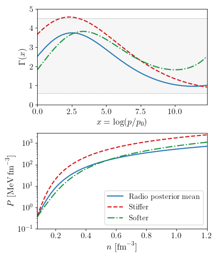
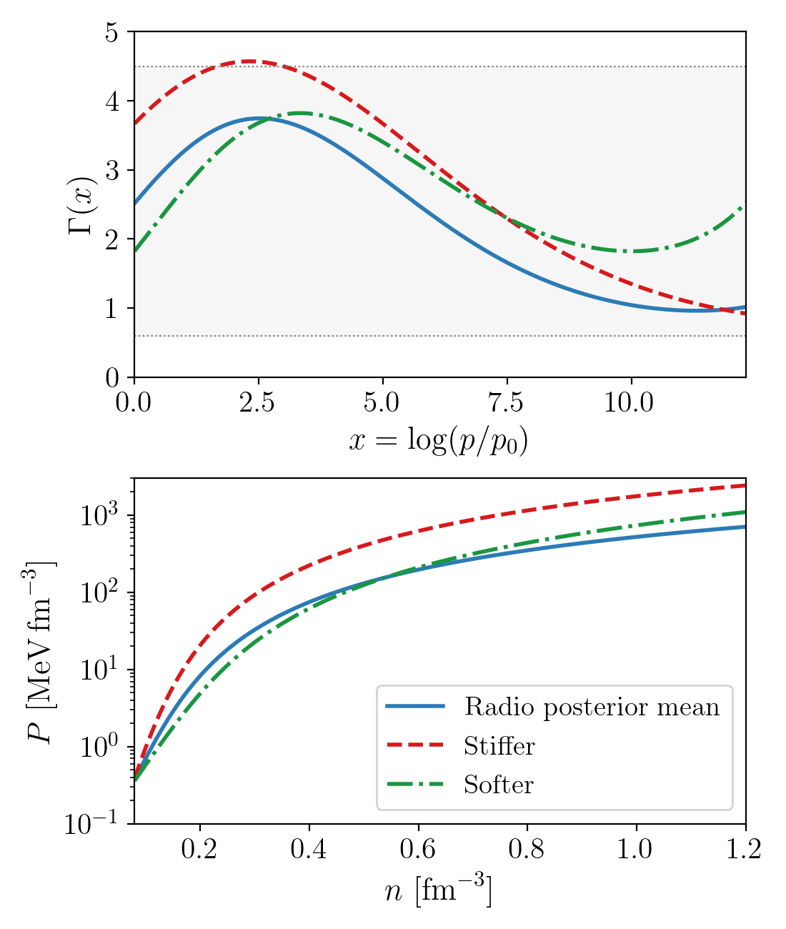
The figure below shows \(\Gamma(x)\) and the pressure-density relation for three representative parameter sets; the grey band marks the valid adiabatic index range. The label ‘radio posterior mean’ refers to the mean spectral coefficients from a radio-timing-only inference run, which are used as the center of the Gaussian reparametrization described in the next section below.
(Source code, png, hires.png, pdf)

Top: adiabatic index \(\Gamma(x)\) across the spectral domain for three representative parameter sets. The grey band marks the valid range \([0.6, 4.5]\). Bottom: the corresponding pressure-density relation above the crust.#
Usage#
Configuration file:
eos:
  type: spectral
  crust_name: SLy
  n_points_high: 100
Prior file:
gamma_0 = UniformPrior(0.2, 2.0, parameter_names=["gamma_0"])
gamma_1 = UniformPrior(-1.6, 1.7, parameter_names=["gamma_1"])
gamma_2 = UniformPrior(-0.6, 0.6, parameter_names=["gamma_2"])
gamma_3 = UniformPrior(-0.02, 0.02, parameter_names=["gamma_3"])
Complete examples are in examples/inference/spectral/.
Reparametrization#
With a flat prior on \((\gamma_0, \gamma_1, \gamma_2, \gamma_3)\), a large fraction of samples produce numerically broken EOS: when \(\Gamma\) drops below 1, the integrating factor \(\mu(x)\) collapses exponentially to zero, causing the energy density to diverge and the subsequent TOV integration to return NaN. This is not a bug — it reflects the fact that much of the flat prior volume corresponds to unphysical high-density matter — but it makes inference inefficient.
A more efficient alternative is to draw the spectral coefficients from a prior that is already
concentrated on physically reasonable EOS. In jester this is achieved with a
Gaussian reparametrization inspired by the posterior from a radio-timing-only inference run.
The idea is that the radio constraints (maximum observed pulsar mass \(\approx 2\,M_\odot\))
already rule out the softest EOS and loosely constrain the spectral coefficients to a
four-dimensional ellipsoid.
A multivariate Gaussian is fitted to this radio posterior by computing the weighted empirical mean
\(\boldsymbol{\mu}_\mathrm{radio}\) and covariance \(\Sigma_\mathrm{radio}\), and then the
Cholesky factor \(L\) of \(\Sigma_\mathrm{radio}\) is widened by a scale factor
\(\sigma_\mathrm{scale} = 1.5\) to remain broader than the radio posterior.
The reparametrized prior then places a standard normal over the whitened coordinates
where \(L_\mathrm{wide} = \sigma_\mathrm{scale}\,L\).
The sampler works entirely in the \(\tilde{\boldsymbol{\gamma}}\) space and the transform
maps back to physical spectral coefficients inside construct_eos().
The numerical values of \(\boldsymbol{\mu}_\mathrm{radio}\) and \(L\) are
hardcoded in SpectralDecomposition_EOS_model and were derived
from a BlackJAX SMC run with radio constraints only using fiducial pulsar masses.
For reference, the hardcoded constants are (rounded to 4 decimal places):
To use the reparametrization, set reparametrized: true in the config and replace the
flat \(\gamma\) priors with a standard MultivariateGaussianPrior:
Configuration file:
eos:
  type: spectral
  crust_name: SLy
  reparametrized: true
Prior file:
spectral_reparam = MultivariateGaussianPrior(
    parameter_names=["gamma_0_tilde", "gamma_1_tilde", "gamma_2_tilde", "gamma_3_tilde"],
)
A complete working example is in examples/inference/spectral_reparam/.
Further resources#
API reference:
jesterTOV.eos.spectral.SpectralDecomposition_EOS_modelPrior class:
jesterTOV.inference.base.prior.MultivariateGaussianPrior
References
Lee Lindblom. Spectral Representations of Neutron-Star Equations of State. Phys. Rev. D, 82:103011, 2010. arXiv:1009.0738, doi:10.1103/PhysRevD.82.103011.